
How to visualize a country outline in Jupyter using GeoPandas, Cartopy & Natural Earth
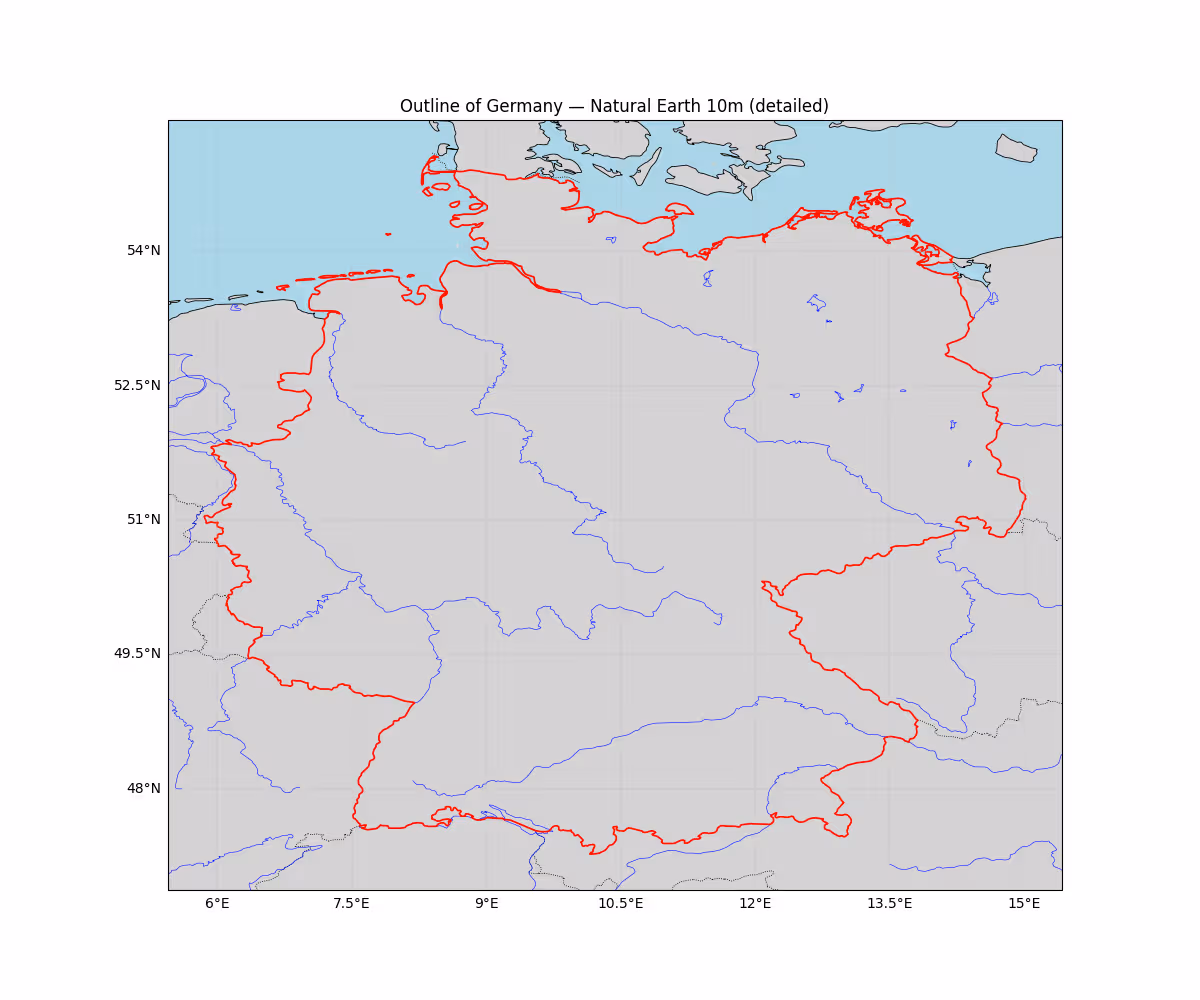
This simple example shows how to visualize a country’s outline in Jupyter. For this example, we’ll show the outline of Germany. To make it more visually appealing, we also add other countries’ outlines and the ocean in the background.
We use the Natural Earth 10m dataset, which is automatically downloaded here. The larger-scale variants such as 1:110M just don’t provide enough resolution at this scale to be visually appealing.
VisualizeCountry.py
# Import required libraries
import cartopy.crs as ccrs
import cartopy.feature as cf
from cartopy.feature import ShapelyFeature
import cartopy.io.shapereader as shpreader
import matplotlib.pyplot as plt
import geopandas as gpd
from shapely.ops import unary_union

# Create the map with Plate Carree projection
proj = ccrs.PlateCarree()
ax = plt.axes(projection=proj)
# We'll pull higher-resolution Natural Earth (10m) where available
# Use the 10m 'admin_0_countries' and coastline/lakes/rivers for detail
try:
    # Read 10m Natural Earth countries and extract Germany geometry via geopandas for better accuracy
    countries = gpd.read_file(shpreader.natural_earth(resolution='10m', category='cultural', name='admin_0_countries'))
    germany = countries[countries['ISO_A3'] == 'DEU'].iloc[0].geometry
    # Buffer by 0 to fix any invalid geometries
    germany = germany.buffer(0)
    # Determine a tight extent from the geometry with a small padding in degrees
    minx, miny, maxx, maxy = germany.bounds
    pad_deg = 0.4
    extent = [minx - pad_deg, maxx + pad_deg, miny - pad_deg, maxy + pad_deg]
    ax.set_extent(extent, crs=ccrs.PlateCarree())

    # Add high-res coastline and borders and lakes/rivers
    # NOTE: All of those are optional - just comment out what you don't need
    ax.add_feature(cf.LAND.with_scale('10m'), facecolor='lightgray')
    ax.add_feature(cf.OCEAN.with_scale('10m'), facecolor='lightblue')
    ax.add_feature(cf.COASTLINE.with_scale('10m'), lw=0.6)
    ax.add_feature(cf.BORDERS.with_scale('10m'), linestyle=':', lw=0.6)
    ax.add_feature(cf.LAKES.with_scale('10m'), facecolor='none', edgecolor='blue', lw=0.4)
    ax.add_feature(cf.RIVERS.with_scale('10m'), edgecolor='blue', lw=0.4)

    # Add Germany polygon with nicer styling
    germany_feature = ShapelyFeature([germany], ccrs.PlateCarree(), facecolor='none', edgecolor='red', linewidth=1.2)
    ax.add_feature(germany_feature)

    # Add gridlines and title
    gl = ax.gridlines(draw_labels=True, linestyle='--', linewidth=0.3)
    gl.top_labels = False
    gl.right_labels = False
    plt.gcf().set_size_inches(12, 10)
    ax.set_title('Outline of Germany — Natural Earth 10m (detailed)')

    plt.show()
except Exception as e:
    print(f"Error: {e}")
    print("Could not load 10m Natural Earth data. Falling back to built-in shapereader records with 110m resolution.")
    try:
        reader = shpreader.Reader(shpreader.natural_earth(resolution='110m', category='cultural', name='admin_0_countries'))
        germany = [c for c in reader.records() if c.attributes['NAME_LONG'] == 'Germany'][0]
        shape_feature = ShapelyFeature([germany.geometry], ccrs.PlateCarree(), facecolor='none', edgecolor='red', lw=2)
        ax.add_feature(cf.COASTLINE, lw=0.5)
        ax.add_feature(cf.BORDERS, linestyle=':', lw=0.5)
        ax.add_feature(shape_feature)
        plt.show()
    except Exception as e2:
print('Fallback also failed:', e2)Check out similar posts by category:
Geoinformatics
If this post helped you, please consider buying me a coffee or donating via PayPal to support research & publishing of new posts on TechOverflow