
寻找最小邮政编码集合以(几乎)完全覆盖一个国家的算法
本文介绍如何使用 Python 和一些常用库,选择一个最小的邮政编码(PLZ)集合来几乎完全覆盖一个国家。示例以德国为例,但该方法可以适配到其他具有类似邮政编码系统的国家。
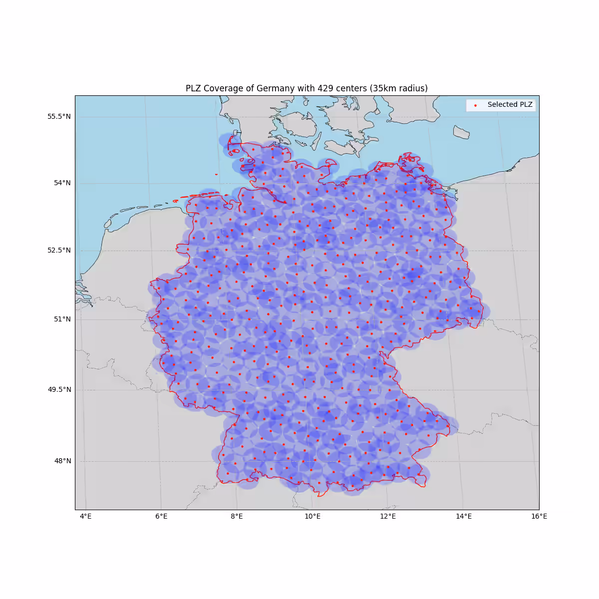
我们这里使用的模型是:在每个选定的邮政编码(即中心)周围绘制一个恒定半径的圆,目标是用尽可能少的圆覆盖尽可能多的国家面积。这是一个经典的优化问题,通常被称为“集合覆盖问题”,属于 NP-hard 问题。因此,我们使用带有一些增强的贪心近似算法,在合理的时间内找到一个较好的解。
该算法可以轻松适配到其他国家,也可以适配到其他兴趣点(POI)集合。
这主要是一个随机算法,因此可能不会产生绝对最优的结果,但在大多数情况下应该非常接近最优。此外,即使在普通笔记本电脑上,它也能在数秒内运行完成(参数与下方示例相同)。
由于此代码以 parquet 文件的形式读取 PLZ 表,请参阅我们之前的文章 从 GeoNames 解析邮政编码和坐标
获取代码,并运行 python parse_de.py -p postleitzahlen.parquet 来创建所需的文件。
结果
使用下方示例用法,我们最终选择了 429 个中心(邮政编码),以每个选定邮政编码周围 35 km 的半径覆盖了德国 99.5% 的面积。
完整源代码
plz-coverage.py
__author__ = "Uli Köhler"
__copyright__ = "Copyright 2025, Uli Köhler"
__license__ = "CC0 1.0 Universal (CC0 1.0) Public Domain Dedication"

import geopandas as gpd
import pandas as pd
import numpy as np
from shapely.geometry import Point
from shapely.ops import unary_union
import matplotlib.pyplot as plt
from tqdm.auto import tqdm
import cartopy.crs as ccrs
import cartopy.feature as cfeature
from cartopy.feature import ShapelyFeature
from sklearn.neighbors import KDTree
import cartopy.io.shapereader as shpreader

# 内联的 PLZ 和国家加载器(自包含)
def load_plz_data(plz_file_path: str) -> pd.DataFrame:
    """从文件路径加载邮政编码表格数据(parquet 或 CSV)。"""
    if plz_file_path.endswith('.parquet') or plz_file_path.endswith('.parq'):
        return pd.read_parquet(plz_file_path)
    if plz_file_path.endswith('.csv') or plz_file_path.endswith('.txt'):
        return pd.read_csv(plz_file_path)
    # 尝试常用读取器作为后备
    try:
        return pd.read_parquet(plz_file_path)
    except Exception:
        try:
            return pd.read_csv(plz_file_path)
        except Exception as exc:
            raise RuntimeError(f'Could not read PLZ data from {plz_file_path}: {exc}') from exc


def create_plz_points(plz_df: pd.DataFrame) -> gpd.GeoDataFrame:
    """从 DataFrame 创建 PLZ 点的 GeoDataFrame。
    期望经度/纬度位于名为 ('lon','lng','longitude') 之一和 ('lat','latitude') 之一的列中。
    同时通过复制常用邮政编码列或回退到索引来确保存在 'PLZ' 列。
    """
    df = plz_df.copy()
    # 容错的坐标列查找
    lon_cols = [c for c in df.columns if c.lower() in ('lon', 'lng', 'longitude')]
    lat_cols = [c for c in df.columns if c.lower() in ('lat', 'latitude')]
    if not lon_cols or not lat_cols:
        raise ValueError('PLZ dataframe must contain lon and lat columns (e.g. lon, lat)')
    lon_col = lon_cols[0]
    lat_col = lat_cols[0]
    df = df.dropna(subset=[lon_col, lat_col]).copy()
    geometry = [Point(xy) for xy in zip(df[lon_col].astype(float), df[lat_col].astype(float))]
    gdf = gpd.GeoDataFrame(df, geometry=geometry, crs="EPSG:4326")
    # 为下游代码保留常规列名
    if 'lon' not in gdf.columns:
        gdf['lon'] = gdf[lon_col].astype(float)
    if 'lat' not in gdf.columns:
        gdf['lat'] = gdf[lat_col].astype(float)

    # 确保存在 PLZ 列(邮政编码)。先尝试常用名称,否则回退到索引作为字符串
    plz_cols = [c for c in gdf.columns if c.lower() in ('plz', 'postal_code', 'postal', 'postleitzahl')]
    if plz_cols:
        gdf['PLZ'] = gdf[plz_cols[0]].astype(str)
    else:
        # 如果有名为 'zip' 或 'postcode' 的数字列,则选择它
        zip_cols = [c for c in gdf.columns if c.lower() in ('zip', 'postcode')]
        if zip_cols:
            gdf['PLZ'] = gdf[zip_cols[0]].astype(str)
        else:
            # 后备:从索引创建 PLZ 以获得稳定标识符
            gdf = gdf.reset_index(drop=False)
            gdf['PLZ'] = gdf['index'].astype(str)
            gdf.drop(columns=['index'], inplace=True)

    return gdf


def load_germany_from_natural_earth() -> object:
    """读取 10m Natural Earth 国家数据并返回德国几何图形(shapely)"""
    # 使用 cartopy 的 shapereader 路径和 geopandas 加载 10m admin_0_countries shapefile
    shp_path = shpreader.natural_earth(resolution='10m', category='cultural', name='admin_0_countries')
    countries = gpd.read_file(shp_path)
    # 尝试常用的 ISO 列名来匹配德国
    iso_cols = [c for c in ('ISO_A3', 'ISO3', 'adm0_a3', 'ADM0_A3', 'iso_a3') if c in countries.columns]
    if iso_cols:
        germany = countries[countries[iso_cols[0]] == 'DEU']
    else:
        # 后备:尝试按 NAME 或 SOVEREIGNT 匹配
        name_cols = [c for c in ('NAME_EN', 'NAME', 'SOVEREIGNT', 'ADMIN') if c in countries.columns]
        if name_cols:
            germany = countries[countries[name_cols[0]].str.contains('Germany', case=False, na=False)]
        else:
            raise RuntimeError('Could not determine ISO or name column in Natural Earth countries')
    if germany.empty:
        raise RuntimeError('Germany geometry not found in Natural Earth countries')
    return germany.iloc[0].geometry


def filter_plz_in_germany(plz_gdf, germany_geometry):
    """筛选位于德国境内的 PLZ 点"""
    plz_gdf = plz_gdf.to_crs("EPSG:3857")  # Web Mercator,用于距离计算
    germany_geometry = gpd.GeoSeries([germany_geometry], crs="EPSG:4326").to_crs("EPSG:3857")[0]

    # 在德国周围创建缓冲区,以包含边境附近的 PLZ
    buffered_germany = germany_geometry.buffer(50000)  # 50km 缓冲区

    # 筛选位于缓冲后德国范围内的 PLZ
    plz_in_germany = plz_gdf[plz_gdf.intersects(buffered_germany)]
    return plz_in_germany


def calculate_coverage(selected_plz, germany_geometry, radius_km=30):
    """计算所选 PLZ 覆盖德国的百分比"""
    radius_m = radius_km * 1000
    coverage = unary_union(selected_plz.geometry.buffer(radius_m))
    germany_geometry = gpd.GeoSeries([germany_geometry], crs="EPSG:4326").to_crs("EPSG:3857")[0]
    covered_area = germany_geometry.intersection(coverage).area
    total_area = germany_geometry.area
    return covered_area / total_area * 100


def _generate_grid_points_in_polygon(polygon_3857, step_m: float) -> np.ndarray:
    """在给定多边形(EPSG:3857)内生成规则网格点 (x, y)。"""
    xmin, ymin, xmax, ymax = polygon_3857.bounds
    xs = np.arange(xmin, xmax + step_m, step_m)
    ys = np.arange(ymin, ymax + step_m, step_m)
    points = []
    # 简单循环对于约 2 万到 6 万个点来说没问题
    for x in xs:
        for y in ys:
            p = Point(x, y)
            if polygon_3857.contains(p):
                points.append((x, y))
    if not points:
        return np.empty((0, 2), dtype=float)
    return np.array(points, dtype=float)


def select_plz_max_coverage(
    plz_gdf: gpd.GeoDataFrame,
    germany_geometry,
    radius_km: float = 30,
    coverage_target: float = 0.99,
    sample_size: int = 300,
    grid_step_km: float = 5.0,
    exclusion_factor: float = 0.75,
    max_steps: int = 10000,
    patience: int = 500,
    validate_every: int = 50,
    random_state: int = 42,
    verbose: bool = True
) -> gpd.GeoDataFrame:
    """
    选择 PLZ 点以最大化覆盖面积(近似)的单一算法。

    使用德国境内(EPSG:3857)的规则网格点作为面积代理。
    贪心随机化:在每一步从剩余候选中抽样一个子集,
    并选择在半径内覆盖最多当前未覆盖网格点的那个。

    增强:
    - 定期精确覆盖检查(unary_union)以避免过早停止。
    - 排除半径以抑制聚集选择:在选定一个中心后,
      丢弃 (exclusion_factor * radius_km) 范围内的所有剩余 PLZ。

    返回:所选 PLZ 点的 GeoDataFrame(EPSG:3857)。
    """
    rng = np.random.default_rng(random_state)

    # 确保投影 CRS 用于距离/面积,并准备几何图形
    work_gdf = plz_gdf.to_crs("EPSG:3857").copy()
    germany_3857 = gpd.GeoSeries([germany_geometry], crs="EPSG:4326").to_crs("EPSG:3857")[0]

    radius_m = float(radius_km) * 1000.0
    exclusion_m = float(exclusion_factor) * radius_m
    grid_step_m = float(grid_step_km) * 1000.0

    # 1) 在德国境内构建网格点作为覆盖代理
    if verbose:
        print(f"Building {grid_step_km:.1f} km grid over Germany for coverage approximation...")
    grid_xy = _generate_grid_points_in_polygon(germany_3857, step_m=grid_step_m)
    if grid_xy.shape[0] == 0:
        raise RuntimeError("Failed to generate grid points inside Germany polygon.")
    if verbose:
        print(f"Grid points: {grid_xy.shape[0]:,}")

    # 2) 在网格上建立 KDTree 以进行快速半径查询
    tree_grid = KDTree(grid_xy, leaf_size=40, metric='euclidean')

    # 3) 为每个 PLZ 候选预计算邻居网格索引
    plz_xy = np.column_stack([work_gdf.geometry.x.values, work_gdf.geometry.y.values])
    if verbose:
        print("Precomputing candidate-to-grid coverage neighborhoods...")
    neighbor_lists = tree_grid.query_radius(plz_xy, r=radius_m, return_distance=False)

    # 3b) 在 PLZ 候选上建立 KDTree 以进行排除过滤
    tree_plz = KDTree(plz_xy, leaf_size=40, metric='euclidean')

    # 4) 在未覆盖网格掩码上进行贪心随机选择循环
    uncovered = np.ones(grid_xy.shape[0], dtype=bool)
    selected_mask = np.zeros(len(work_gdf), dtype=bool)
    active_mask = np.ones(len(work_gdf), dtype=bool)  # 仍然可用的候选
    no_improve_steps = 0

    pbar = tqdm(total=max_steps, disable=not verbose, desc="Selecting centers (max-coverage)")
    for step in range(max_steps):
        pbar.update(1)

        # 定期精确覆盖检查
        if step % validate_every == 0 and selected_mask.any():
            selected_tmp = work_gdf.loc[selected_mask]
            exact_cov = calculate_coverage(selected_tmp, germany_geometry, radius_km) / 100.0
            if step % (validate_every * 2) == 0:
                pbar.set_postfix_str(f"exact~{exact_cov*100:.1f}%")
            if exact_cov >= coverage_target:
                break

        # 在网格上近似覆盖比例
        covered_frac = 1.0 - (uncovered.sum() / uncovered.size)
        if covered_frac >= coverage_target and selected_mask.any():
            selected_tmp = work_gdf.loc[selected_mask]
            exact_cov = calculate_coverage(selected_tmp, germany_geometry, radius_km) / 100.0
            if exact_cov >= coverage_target:
                break

        remaining_idx = np.flatnonzero(active_mask)
        if remaining_idx.size == 0:
            break

        # 从活跃集合中抽样候选
        k = int(min(sample_size, remaining_idx.size))
        sample = rng.choice(remaining_idx, size=k, replace=False) if k > 0 else []

        # 在网格上评估边际增益
        best_gain = 0
        best_idx = None
        for idx in sample:
            neigh = neighbor_lists[idx]
            if neigh.size == 0:
                continue
            gain = int(uncovered[neigh].sum())
            if gain > best_gain:
                best_gain = gain
                best_idx = idx

        if best_idx is None or best_gain == 0:
            no_improve_steps += 1
            if no_improve_steps >= patience:
                break
            else:
                continue

        # 接受最佳候选
        selected_mask[best_idx] = True
        # 将网格点标记为已覆盖
        uncovered[neighbor_lists[best_idx]] = False
        # 排除附近的 PLZ 以减少聚集
        if exclusion_m > 0:
            near = tree_plz.query_radius(plz_xy[[best_idx]], r=exclusion_m, return_distance=False)[0]
            active_mask[near] = False
        # 同时移除所选索引
        active_mask[best_idx] = False
        no_improve_steps = 0

    pbar.close()

    selected = work_gdf.loc[selected_mask].copy()
    selected = selected.set_crs("EPSG:3857")
    return selected


def visualize_coverage(selected_plz, germany_geometry, radius_km=30):
    """使用 Cartopy 可视化覆盖情况"""
    # 转换为 WGS84 以便可视化
    selected_plz = selected_plz.to_crs("EPSG:4326")
    germany_geometry = gpd.GeoSeries([germany_geometry], crs="EPSG:4326").to_crs("EPSG:4326")[0]

    # 使用 Cartopy 投影创建图形
    fig = plt.figure(figsize=(12, 12))
    ax = fig.add_subplot(1, 1, 1, projection=ccrs.EqualEarth())

    # 添加地图要素
    ax.add_feature(cfeature.LAND, facecolor='lightgray')
    ax.add_feature(cfeature.OCEAN, facecolor='lightblue')
    ax.add_feature(cfeature.COASTLINE, linewidth=0.5)
    ax.add_feature(cfeature.BORDERS, linestyle=':', linewidth=0.5)

    # 为德国创建 ShapelyFeature
    germany_feature = ShapelyFeature([germany_geometry], ccrs.PlateCarree(), facecolor='none', edgecolor='red', linewidth=1)
    ax.add_feature(germany_feature)

    # 创建并绘制圆(现在为所有 PLZ)
    radius_m = radius_km * 1000
    buffers_3857 = gpd.GeoSeries(selected_plz.geometry).to_crs("EPSG:3857").buffer(radius_m)
    buffers_4326 = gpd.GeoSeries(buffers_3857, crs="EPSG:3857").to_crs("EPSG:4326")

    # 单独绘制每个缓冲区,使重叠部分渲染为分层透明度
    for geom in buffers_4326:
        ax.add_geometries([geom], crs=ccrs.PlateCarree(), facecolor='blue', edgecolor='none', alpha=0.2, zorder=2)

    # 在顶层绘制所选 PLZ 点
    ax.scatter(selected_plz.geometry.x, selected_plz.geometry.y, color='red', s=5, transform=ccrs.PlateCarree(), label='Selected PLZ', zorder=3)

    # 设置范围为德国并留有一些边距
    ax.set_extent([4, 16, 47, 56], crs=ccrs.PlateCarree())

    # 添加网格线
    gl = ax.gridlines(draw_labels=True, linestyle='--')
    gl.top_labels = False
    gl.right_labels = False

    plt.title(f"PLZ Coverage of Germany with {len(selected_plz)} centers ({radius_km}km radius)")
    plt.legend(loc='upper right')
    plt.show()


def run_analysis(plz_file_path, radius_km=30, coverage_target=0.99):
    """使用单一最大覆盖算法进行分析的主函数"""
    # 从 Natural Earth 加载德国几何图形
    print("Loading Germany geometry from Natural Earth...")
    germany_geometry = load_germany_from_natural_earth()

    # 加载并处理 PLZ 数据
    print("Loading PLZ data...")
    plz_df = load_plz_data(plz_file_path)
    print(f"Loaded {len(plz_df)} German postal codes")

    plz_gdf = create_plz_points(plz_df)

    print("Filtering PLZ within Germany...")
    plz_in_germany = filter_plz_in_germany(plz_gdf, germany_geometry)
    print(f"Found {len(plz_in_germany)} PLZ within or near Germany")

    # 使用单一算法选择 PLZ 中心
    print("Selecting PLZ centers with max-coverage algorithm...")
    selected_plz = select_plz_max_coverage(
        plz_in_germany, germany_geometry, radius_km=radius_km, coverage_target=coverage_target, sample_size=300, grid_step_km=2.0, exclusion_factor=0.75, max_steps=10000, patience=500, validate_every=50, random_state=42, verbose=True
    )

    # 计算覆盖率(精确,单次联合)
    coverage_percent = calculate_coverage(selected_plz, germany_geometry, radius_km)
    print(f"\nSelected {len(selected_plz)} PLZ centers covering {coverage_percent:.1f}% of Germany")

    # 可视化覆盖情况
    visualize_coverage(selected_plz, germany_geometry=germany_geometry, radius_km=radius_km)

    # 防御性地返回结果:仅包含存在的列
    sel = selected_plz.to_crs("EPSG:4326")
    desired = ['PLZ', 'lat', 'lon', 'geometry']
    available = [c for c in desired if c in sel.columns or c == 'geometry']
    # 确保存在 geometry
    if 'geometry' not in available:
        available.append('geometry')

    return {
        'selected_plz': sel[available],
        'coverage_percent': coverage_percent,
        'total_plz_used': len(selected_plz)
}此代码适用于 Jupyter Notebook。
示例用法
example-usage.py
results = run_analysis(
    plz_file_path="postleitzahlen.parquet",
    radius_km=35,
    coverage_target=0.995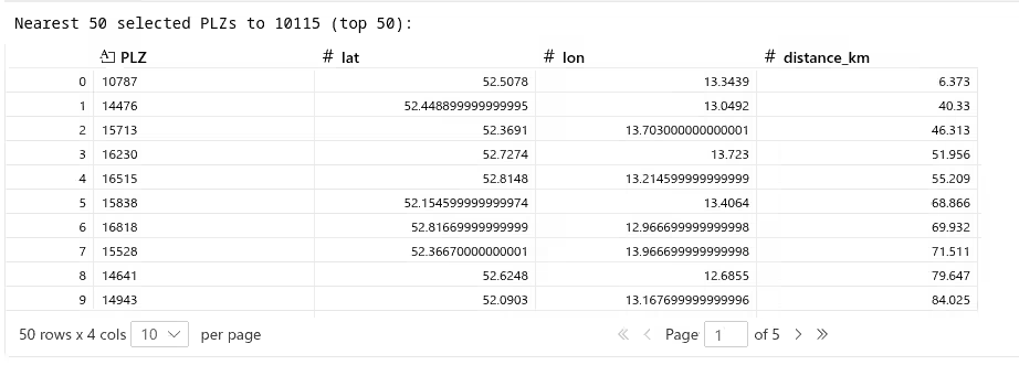
)如何查找与给定邮政编码最近的结果 PLZ
这个可选的附加功能接受某个地点的参考 PLZ 编码,并生成一个包含距离最近的 50 个所选 PLZ 的 DataFrame。 这假设你已使用 Jupyter Notebook 运行了前面的代码。
find_nearest_plz.py
# 单元格:查找与给定 PLZ(示例:63110)最近的 50 个所选 PLZ
plz_code = '10176'

# 确保我们有可用的所选结果;如果没有,则运行一次分析(轻量级防护)
if 'results' not in globals():
    print('`results` not found in the notebook namespace — running `run_analysis` (this may take time)')
    results = run_analysis(plz_file_path="postleitzahlen.parquet", radius_km=35, coverage_target=0.995)

selected = results['selected_plz']

# 加载完整 PLZ 表以定位参考 PLZ 坐标
plz_df = load_plz_data("postleitzahlen.parquet")
plz_gdf = create_plz_points(plz_df)

# 尝试对 PLZ 进行精确匹配,否则进行前缀匹配
ref = plz_gdf[plz_gdf['PLZ'].astype(str) == str(plz_code)]
if ref.empty:
    ref = plz_gdf[plz_gdf['PLZ'].astype(str).str.startswith(str(plz_code))]

if ref.empty:
    raise ValueError(f"Reference PLZ {plz_code} not found in PLZ dataset")

ref_point = ref.iloc[0].geometry

# 将两者重新投影到投影 CRS 以获得以米为单位的距离(EPSG:3857)
selected_3857 = selected.to_crs("EPSG:3857").copy()
ref_3857 = gpd.GeoSeries([ref_point], crs="EPSG:4326").to_crs("EPSG:3857")[0]

# 计算距离(米)
selected_3857['distance_m'] = selected_3857.geometry.distance(ref_3857)

# 如果参考 PLZ 本身就在所选集合中,则排除它,以便我们获得最近的其他中心
if 'PLZ' in selected_3857.columns:
    selected_for_sort = selected_3857[selected_3857['PLZ'].astype(str) != str(plz_code)]
else:
    selected_for_sort = selected_3857

# 取最近的 50 个
nearest = selected_for_sort.nsmallest(50, 'distance_m').copy()

# 转换回地理坐标并准备友好的 DataFrame
nearest_geo = nearest.to_crs("EPSG:4326")
nearest_geo['lat'] = nearest_geo.geometry.y
nearest_geo['lon'] = nearest_geo.geometry.x
nearest_geo['distance_km'] = (nearest_geo['distance_m'] / 1000.0).round(3)

# 选择要显示的列:优先使用人类可读字段(如果存在)
prefer_columns = ['PLZ', 'name', 'place', 'Ortsteil', 'stadtteil', 'place_name', 'lat', 'lon', 'distance_km']
available = [c for c in prefer_columns if c in nearest_geo.columns]
# 如果没有任何首选名称列存在,则显示所有非几何列
if not available:
    available = [c for c in nearest_geo.columns if c != 'geometry']

nearest_50_df = nearest_geo[available].reset_index(drop=True)

print(f"Nearest {len(nearest_50_df)} selected PLZs to {plz_code} (top {min(50, len(nearest_50_df))}):")
nearest_50_df.head(50) # 显示 DataFrameCheck out similar posts by category:
Algorithms, Geoinformatics
If this post helped you, please consider buying me a coffee or donating via PayPal to support research & publishing of new posts on TechOverflow